API documentation

Index

FEMBase.AbstractField — Type.

AbstractField

Abstract supertype for all fields in JuliaFEM.

source

FEMBase.Assembly — Type.

General linearized problem to solve (K₁+K₂)Δu + C1'Δλ = f₁+f₂ C2Δu + DΔλ = g

source

FEMBase.CVTV — Type.

CVTV <: AbstractField

Continuous, variable, time variant field.

Example

julia> f = CVTV((xi,t) -> xi*t)
FEMBase.CVTV(#1)

source

FEMBase.DCTI — Type.

DCTI{T} <: AbstractField

Discrete, constant, time-invariant field.

This field is constant in both spatial direction and time direction, i.e. df/dX = 0 and df/dt = 0.

Example

julia> DCTI(1)
FEMBase.DCTI{Int64}(1)

source

FEMBase.DCTV — Type.

DCTV{T} <: AbstractField

Discrete, constant, time variant field. This type of field can change in time direction but not in spatial direction.

Example

Field having value 5 at time 0.0 and value 10 at time 1.0:

julia> DCTV(0.0 => 5, 1.0 => 10)
FEMBase.DCTV{Int64}(Pair{Float64,Int64}[0.0=>5, 1.0=>10])

source

FEMBase.DVTI — Type.

DVTI{N,T} <: AbstractField

Discrete, variable, time-invariant field.

This is constant in time direction, but not in spatial direction, i.e. df/dt = 0 but df/dX != 0. The basic structure of data is Tuple, and it is implicitly assumed that length of field matches to the number of shape functions, so that interpolation in spatial direction works.

Example

julia> DVTI(1, 2, 3)
FEMBase.DVTI{3,Int64}((1, 2, 3))

source

FEMBase.DVTId — Type.

DVTId(X::Dict)

Discrete, variable, time invariant dictionary field.

source

FEMBase.DVTV — Type.

DVTV{N,T} <: AbstractField

Discrete, variable, time variant field. The most general discrete field can change in both temporal and spatial direction.

Example

julia> DVTV(0.0 => (1, 2), 1.0 => (2, 3))
FEMBase.DVTV{2,Int64}(Pair{Float64,Tuple{Int64,Int64}}[0.0=>(1, 2), 1.0=>(2, 3)])

source

FEMBase.DVTVd — Type.

DVTVd(time => data::Dict)

Discrete, variable, time variant dictionary field.

source

FEMBase.Element — Method.

Element(element_type, connectivity_vector)

Construct a new element where element_type is the type of the element and connectivity_vector is the vector of nodes that the element is connected to.

Examples

In the example a new element (E in the figure below) of type Tri3 is created. This spesific element connects to nodes 89, 43, 12 in the finite element mesh.

element = Element(Tri3, [89, 43, 12])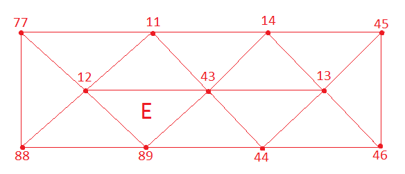

source

FEMBase.Problem — Type.

Defines types for Problem variables.

Examples

The type of 'elements' is Vector{Element}

Add elements into the Problem element list.

a = [1, 2, 3]
Problem.elements = a

source

FEMBase.Problem — Method.

Problem(problem_type, problem_name::String, problem_dimension)

Construct a new field problem where problem_type is the type of the problem (Elasticity, Dirichlet, etc.), problem_name is the name of the problem and problem_dimension is the number of DOF:s in one node (2 in a 2D problem, 3 in an elastic 3D problem, 6 in a 3D beam problem, etc.).

Examples

Create a vector-valued (dim=3) elasticity problem:

prob1 = Problem(Elasticity, "this is my problem", 3)

source

FEMBase.Problem — Method.

Construct a new boundary problem.

Examples

Create a Dirichlet boundary problem for a vector-valued (dim=3) elasticity problem.

julia> bc1 = Problem(Dirichlet, "support", 3, "displacement") solver.

source

FEMBase.add! — Function.

Add new data to COO Sparse vector.

source

FEMBase.add! — Method.

Add local element matrix to sparse matrix. This basically does:

A[dofs1, dofs2] = A[dofs1, dofs2] + data

Example

S = [3, 4] M = [6, 7, 8] data = Float64[5 6 7; 8 9 10] A = SparseMatrixCOO() add!(A, S, M, data) full(A)

4x8 Array{Float64,2}: 0.0 0.0 0.0 0.0 0.0 0.0 0.0 0.0 0.0 0.0 0.0 0.0 0.0 0.0 0.0 0.0 0.0 0.0 0.0 0.0 0.0 5.0 6.0 7.0 0.0 0.0 0.0 0.0 0.0 8.0 9.0 10.0

source

FEMBase.add! — Method.

Add sparse matrix of CSC to COO.

source

FEMBase.add! — Method.

Add SparseVector to SparseVectorCOO.

source

FEMBase.add_elements! — Method.

add_elements!(problem::Problem, elements)

Add new elements into the problem.

source

FEMBase.assemble_mass_matrix! — Method.

assemble_mass_matrix!(problem, elements::Vector{Element{Tet10}}, time)

Assemble Tet10 mass matrices using special method. If Tet10 has constant metric if can be integrated analytically to gain performance.

source

FEMBase.field — Method.

field(x)

Create new field. Field type is deduced from data type.

source

FEMBase.get_gdofs — Method.

Return global degrees of freedom for element.

Notes

First look dofs from problem.dofmap, it not found, update dofmap from element.element connectivity using formula gdofs = [dim*(nid-1)+j for j=1:dim]

look element dofs from problem.dofmap
if not found, use element.connectivity to update dofmap and 1.

source

FEMBase.get_integration_points — Method.

This is a special case, temporarily change order of integration scheme mainly for mass matrix.

source

FEMBase.get_local_coordinates — Method.

Find inverse isoparametric mapping of element.

source

FEMBase.get_nonzero_rows — Method.

Find all nonzero rows from sparse matrix.

Returns

Ordered list of row indices.

source

FEMBase.get_parent_field_name — Method.

Return the name of the parent field of this (boundary) problem.

source

FEMBase.get_unknown_field_dimension — Method.

get_unknown_field_dimension(problem)

Return the dimension of the unknown field of this problem.

source

FEMBase.get_unknown_field_name — Method.

Return the name of the unknown field of this problem.

source

FEMBase.get_unknown_field_name — Method.

get_unknown_field_name(problem)

Default function if unknown field name is not defined for some problem.

source

FEMBase.group_by_element_type — Method.

group_by_element_type(elements::Vector{Element})

Given a vector of elements, group elements by element type to several vectors. Returns a dictionary, where key is the element type and value is a vector containing all elements of type element_type.

source

FEMBase.initialize! — Method.

function initialize!(problem_type, element_name, time)

Initialize the element ready for calculation, where problem_type is the type of the problem (Elasticity, Dirichlet, etc.), element_name is the name of a constructed element (see Element(element_type, connectivity_vector)) and time is the starting time of the initializing process.

source

FEMBase.inside — Method.

Test is X inside element.

source

FEMBase.optimize! — Method.

Combine (I,J,V) values if possible to reduce memory usage.

source

FEMBase.resize_sparse — Method.

Resize sparse matrix A to (higher) dimension n x m.

source

FEMBase.resize_sparsevec — Method.

Resize sparse vector b to (higher) dimension n.

source

FEMBase.update! — Method.

update!(problem, assembly, u, la)

Update the problem solution vector for assembly.

source

FEMBase.update! — Method.

update!(field, data)

Update new value to field.

source

FEMBase.update! — Method.

update!(problem, assembly, elements, time)

Update a solution from the assebly to elements.

source

FEMBase.update! — Method.

update!(problem.properties, attr...)

Update properties for a problem.

Example

update!(body.properties, "finite_strain" => "false")

source

FEMBasis.interpolate — Method.

interpolate(a, b)

A helper function for interpolate routines. Given iterables a and b, calculate c = aᵢbᵢ. Length of a can be less than b, but not vice versa.

source

FEMBasis.interpolate — Method.

interpolate(element, field_name, time)

Interpolate field field_name from element at given time.

Example

element = Element(Seg2, [1, 2])
data1 = Dict(1 => 1.0, 2 => 2.0)
data2 = Dict(1 => 2.0, 2 => 3.0)
update!(element, "my field", 0.0 => data1)
update!(element, "my field", 1.0 => data2)
interpolate(element, "my field", 0.5)

# output

(1.5, 2.5)

source

FEMBasis.interpolate — Method.

interpolate(field, time)

Interpolate field in time direction.

Examples

For time invariant fields DCTI, DVTI, DVTId solution is trivially the data inside field as fields does not depend from the time:

julia> a = field(1.0)
FEMBase.DCTI{Float64}(1.0)

julia> interpolate(a, 0.0)
1.0

julia> a = field((1.0, 2.0))
FEMBase.DVTI{2,Float64}((1.0, 2.0))

julia> interpolate(a, 0.0)
(1.0, 2.0)

julia> a = field(1=>1.0, 2=>2.0)
FEMBase.DVTId{Float64}(Dict(2=>2.0,1=>1.0))

julia> interpolate(a, 0.0)
Dict{Int64,Float64} with 2 entries:
  2 => 2.0
  1 => 1.0

DVTId trivial solution is returned. For time variant fields DCTV, DVTV, DVTVd linear interpolation is performed.

Other notes

First algorithm checks that is time out of range, i.e. time is smaller than time of first frame or larger than last frame. If that is the case, return first or last frame. Secondly algorithm finds is given time exact match to time of some frame and return that frame. At last, we find correct bin so that t0 < time < t1 and use linear interpolation.

source

Base.SparseArrays.sparse — Method.

Convert from COO format to CSC.

Parameters

tol used to drop near zero values less than tol.

source

Base.haskey — Method.

Check existence of field.

source

Base.isapprox — Method.

Approximative comparison of two matricse A and B.

source

Base.length — Method.

length(element)

Return the length of basis (number of nodes).

source

Base.size — Method.

size(element)

Return the size of basis (dim, nnodes).

source

FEMBase.assemble_elements! — Method.

assemble_elements!(problem, assembly, elements, time)

Assemble elements for problem.

This should be overridden with own assemble_elements!-implementation.

source

FEMBase.get_global_solution — Method.

get_global_solution(problem, assembly)

Return a global solution (u, la) for a problem.

Notes

If the length of solution vector != number of nodes, i.e. the field dimension is something else than 1, reshape vectors so that their length matches to the number of nodes. This helps to get nodal results easily.

source

FEMBasis.BasisInfo — Type.

Data type for fast FEM.

source

FEMBasis.BasisInfo — Method.

Initialization of data type BasisInfo.

Examples


BasisInfo(Tri3)

# output

FEMBasis.BasisInfo{FEMBasis.Tri3,Float64}([0.0 0.0 0.0], [0.0 0.0 0.0; 0.0 0.0 0.0], [0.0 0.0 0.0; 0.0 0.0 0.0], [0.0 0.0; 0.0 0.0], [0.0 0.0; 0.0 0.0], 0.0)

source

FEMBasis.NSeg — Type.

NURBS segment.

source

FEMBasis.eval_basis! — Method.

Evaluate basis, gradient and so on for some point xi.

Examples


b = BasisInfo(Quad4)
X = ((0.0,0.0), (1.0,0.0), (1.0,1.0), (0.0,1.0))
xi = (0.0, 0.0)
eval_basis!(b, X, xi)

# output

FEMBasis.BasisInfo{FEMBasis.Quad4,Float64}([0.25 0.25 0.25 0.25], [-0.25 0.25 0.25 -0.25; -0.25 -0.25 0.25 0.25], [-0.5 0.5 0.5 -0.5; -0.5 -0.5 0.5 0.5], [0.5 0.0; 0.0 0.5], [2.0 -0.0; -0.0 2.0], 0.25)

source

FEMBasis.grad! — Method.

grad!(bi, gradu, u)

Evalute gradient ∂u/∂X and store result to matrix gradu. It is assumed that eval_basis! has been already run to bi so it already contains all necessary matrices evaluated with some X and xi.

Example

First setup and evaluate basis using eval_basis!:

B = BasisInfo(Quad4)
X = ((0.0,0.0), (1.0,0.0), (1.0,1.0), (0.0,1.0))
xi = (0.0, 0.0)
eval_basis!(B, X, xi)

# output

FEMBasis.BasisInfo{FEMBasis.Quad4,Float64}([0.25 0.25 0.25 0.25], [-0.25 0.25 0.25 -0.25; -0.25 -0.25 0.25 0.25], [-0.5 0.5 0.5 -0.5; -0.5 -0.5 0.5 0.5], [0.5 0.0; 0.0 0.5], [2.0 -0.0; -0.0 2.0], 0.25)

Next, calculate gradient of u:

u = ((0.0, 0.0), (1.0, -1.0), (2.0, 3.0), (0.0, 0.0))
gradu = zeros(2, 2)
grad!(B, gradu, u)

# output

2×2 Array{Float64,2}:
 1.5  0.5
 1.0  2.0

source

FEMBasis.grad — Method.

grad(B, T, X, xi)

Calculate gradient of T with respect to X in point xi using basis B.

Example

B = Quad4()
X = ([0.0, 0.0], [1.0, 0.0], [1.0, 1.0], [0.0, 1.0])
u = ([0.0, 0.0], [1.0, -1.0], [2.0, 3.0], [0.0, 0.0])
grad(B, u, X, (0.0, 0.0))

# output

2×2 Array{Float64,2}:
 1.5  0.5
 1.0  2.0

source

FEMBasis.grad — Method.

grad(B, X, xi)

Given basis B, calculate gradient dB/dX at xi.

Example

B = Quad4()
X = ([0.0, 0.0], [1.0, 0.0], [1.0, 1.0], [0.0, 1.0])
grad(B, X, (0.0, 0.0))

# output

2×4 Array{Float64,2}:
 -0.5   0.5  0.5  -0.5
 -0.5  -0.5  0.5   0.5

source

FEMBasis.interpolate — Method.

interpolate(B, T, xi)

Given basis B, interpolate T at xi.

Example

B = Quad4()
X = ((0.0, 0.0), (1.0, 0.0), (1.0, 1.0), (0.0, 1.0))
T = (1.0, 2.0, 3.0, 4.0)
interpolate(B, T, (0.0, 0.0))

# output

2.5

source

FEMBasis.jacobian — Method.

jacobian(B, X, xi)

Given basis B, calculate jacobian at xi.

Example

B = Quad4()
X = ([0.0, 0.0], [1.0, 0.0], [1.0, 1.0], [0.0, 1.0])
jacobian(B, X, (0.0, 0.0))

# output

2×2 Array{Float64,2}:
 0.5  0.0
 0.0  0.5

source

FEMBasis.calculate_basis_coefficients — Method.

function calculate_basis_coefficients(polynomial::String, coordinates::Vararg{Tuple})

Calculate "interpolate coefficient matrix" for some polynomial p.

Examples

That is, if we have polynomial p = 1 + u + v and coordinates (0,0), (1,0), (0,1), we find A*p such that first row is the first coordinate, second row is second coordinate and so on:

julia> p = "1 + u + w"
julia> X = ((0.0,0.0), (1.0,0.0), (0.0,1.0))
julia> calculate_basis_coefficient(p, X)
[1.0 0.0 0.0 # <-- p(0.0,0.0) = 1.0     = [1.0 0.0 0.0] * [1.0, u, v]
 1.0 1.0 0.0 # <-- p(1.0,0.0) = 1.0 + u = [1.0 1.0 0.0] * [1.0, u, v]
 1.0 0.0 1.0] # <- p(0.0,1.0) = 1.0 + v = [1.0 0.0 1.0] * [1.0, u, v]

source

FEMBasis.calculate_interpolation_polynomial_derivatives — Method.

Calculate derivatives of basis functions with respect to parameters u, v, w.

source

FEMBasis.calculate_interpolation_polynomials — Method.

source

FEMQuad.get_quadrature_points — Method.

Gauss-Legendre quadrature, 1 point rule on hexahedron.

source

FEMQuad.get_quadrature_points — Method.

Gauss-Legendre quadrature, 243 point rule on quadrilateral.

source